Manually building the Top 5000 Census Surname spreadsheet

Go to the index page for the census-surname lessons:

Learning spreadsheets with Census Surname data

Getting started

As you get better with data and computation, you should avoid work that require manual steps such as pointing-and-clicking with graphical software. If such work causes world-famous Harvard economists to stumble, then why not you?

I’ll make an exception for this Census surname data walkthrough. I hate manual copying-pasting, but it’s only 2 different spreadsheets, and it’s good practice just in case you don’t know some of the point-and-click tricks.

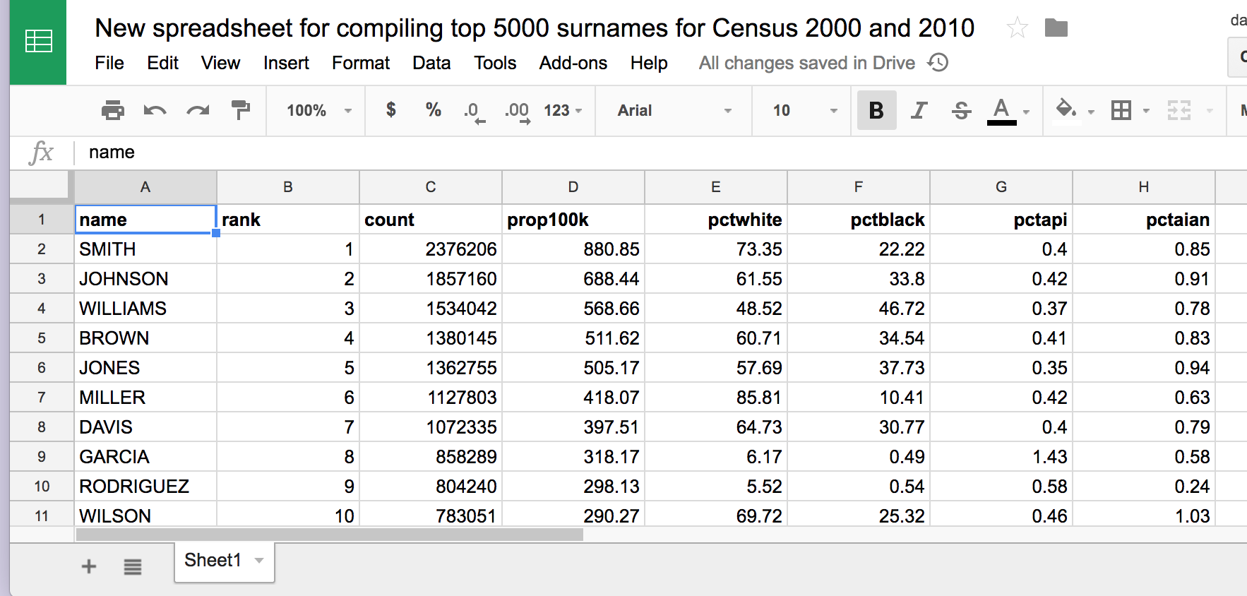
First, create a new, blank spreadsheet. This spreadsheet is where you will be compiling the two Census datasets.

For your convenience, the URLs to the Google Sheets with the 2000 and 2010 surname data:

Census 2010 surnames Google Sheet

Census 2000 surnames Google Sheet

(if you created your own version of the cumulative prop100k column, I advise you to just delete it for now. You won’t need it for later exercises.)

Just to make things easier to follow, and more importantly, to trace back for errors, I’ll break the work into simple, standalone steps:

1. Copy the top 5,000 surnames from the 2000 Census data (plus headers)
2. Paste them into the empty tab of the empty spreadsheet
3. Insert a new column (from the left side) and name it year
4. Auto-fill the year column with 2000.
5. Repeat steps 1 through 4, with a separate tab, for the year 2010 data.

Copy-pasting data from spreadsheets

You probably already know how to copy-and-paste things. But in data work, manual copy-pasting can be the easiest thing to mess up and the hardest mistake to recover from. Not least because if you do mess up – such as not highlighting all of the data you intended to copy/paste – it’s the kind of mistake that you wouldn’t have noticed at the time.

This section is meant to be a quick best-click-practices walkthrough. Hopefully you already know the tricks. If not, hopefully they save you some serious grief in the future!

Efficient row highlighting and selection

OK, open your copy of the Census 2000 surnames Google Sheet. It should already be sorted in ascending order of rank. The first row – i.e. the header row – should also be “frozen”. That is, the headers/column names remain visible as you scroll down the entire dataset.

Scroll your way down to the 5000th-or-so row, whatever row has a rank of 5000. There doesn’t seem to be a power-trick to jump to a given row, unfortunately. The quickest way seems to be via dragging the scroll bar.

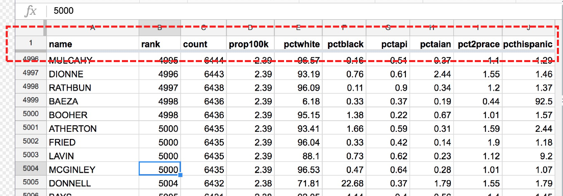
If the header row is frozen, which it should be, the column names should still be visible even though you’re 5,000 rows deep – or rather, 5,004 rows since several names in the 2000 Census data are tied at the 5,000th rank:

Selecting an entire row with a click

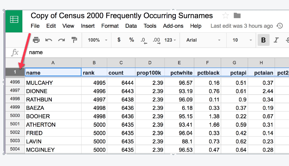
The quickest way to select an entire row, without having to worry about selecting individual columns, is to click the row label – the box/button on the far-left of the spreadsheet. For the header row, the row label has the label of 1.

Click that label will highlight and select the entire row:

Use the Shift-key to select an entire range

Now we want to expand the selection to include every row between the header row to row 5,004.

First, hold down your Shift key. This is how you let the software know that the next click you make is meant to expand the current selection, not be a new selection.

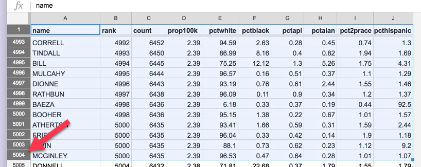
Just like how you selected the entire header row by clicking on the row-label on the left-side of the spreadsheet, do that with row 5004 – again, while holding down the Shift key:

If you scroll up and down the spreadsheet, you should see that all the rows between the header and the desired ending row are highlighted.

Copy to clipboard

If you haven’t mastered the keyboard shortcut for Copy, get started now – using the mouse is too unreliable:

• Windows: Ctrl + C
• OSX: Command + C

Paste to spreadsheet

Switch over to the new spreadsheet you created with its first, empty sheet.

Select the most top-left cell, i.e. A1, and paste via the keyboard-shortcut:

• Windows: Ctrl + V
• OSX: Command + V

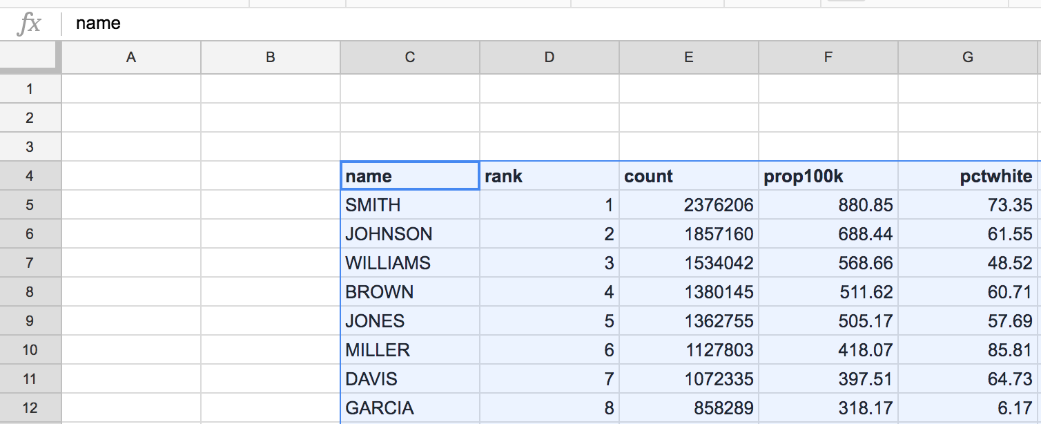
Your system/browser may seem to hang (it’s a lot of data being pasted). If you didn’t select the top-left most cell, you’ll end up with this disaster:

Otherwise, you should have this:

Tidying up

By doing a direct pasting of content, the new spreadsheet should have similar styles (bolded headers). But you’ll probably have to re-freeze the header row. It’s not a big deal in the intermediate steps but might as well do it out of habit.

Also, give the tab of this now-populated sheet a name, something like “Census 2000”.

Our next step is to alter the dataset by adding a new column for year.

Wrangling data means adding to the data

The surname data, as published by the Census, doesn’t contain a column that tells us the year for each surname row. Why not? Think of it from the Census’s perspective. They published the data on a page about the Census 2000, titled: Frequently Occurring Surnames from the Census 2000.

Presumably, everyone who downloads and opens the spreadsheet knows that it is data for the Census 2000.

However, what the Census Bureau didn’t anticipate – or doesn’t have to care about – is that someone, years after 2000 (and 2010). might want to combine the data from the 2000 and 2010 publications.

If we were to copy-pate the Census 2010 surname data into our existing 2000 tab, we wouldn’t be able to tell the difference between the two datasets, especially if we re-sorted the data.

Solving this problem is easy from a technical standpoint. We just need to create a new column for year, which we manually fill with the appropriate year. It’s as easy as it sounds. But for folks new to data wrangling, the idea of augmenting existing data, even with a repetitive literal value (such as the number 2000), doesn’t seem like a solution.

Insert/add the year column

I suggest making year be the very first column of the dataset.

Just in case you need a review on how to insert a new column…

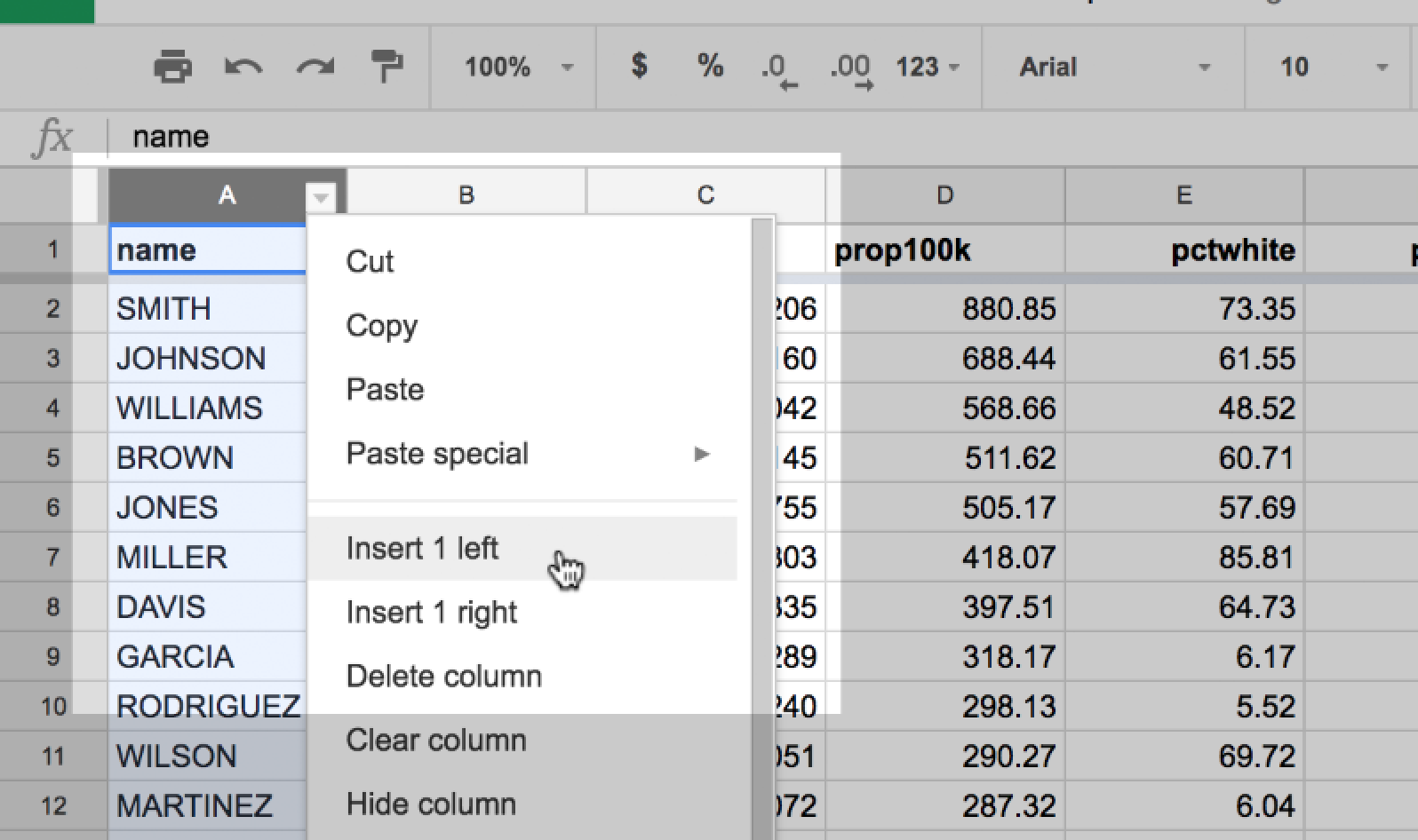
The easiest way to insert a new column relative to an existing one is to hover your mouse over the column-label. In this case, I want to insert a column to the left of Column A, so I hover my mouse pointer over the label A, which brings up a dropdown icon:

Click that icon to reveal the context menu. The action we’re interested in is Insert 1 left:

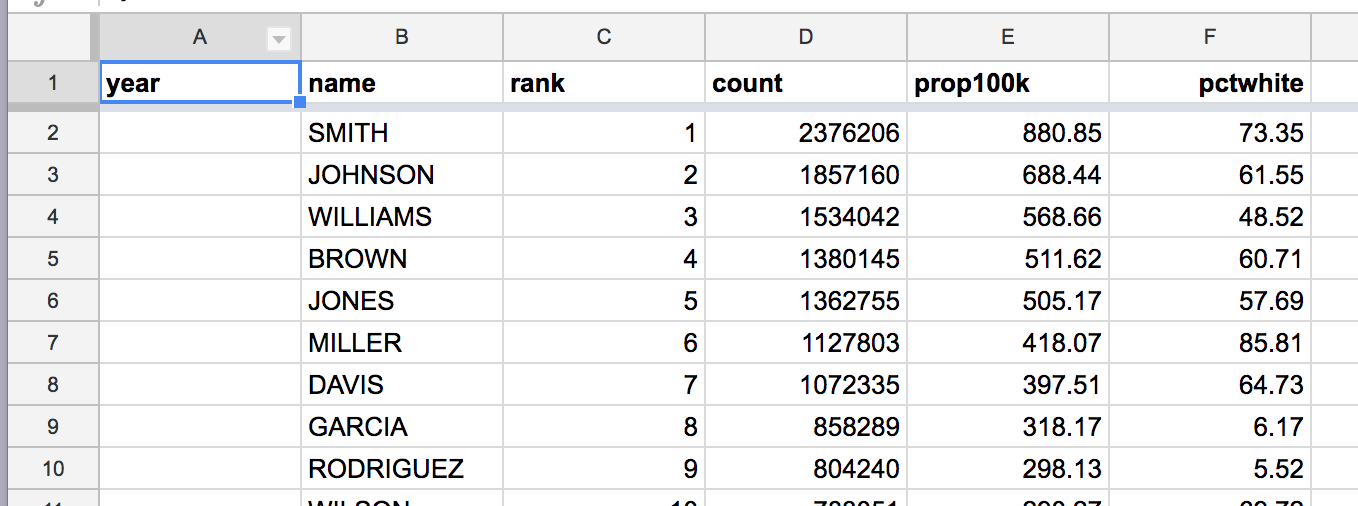
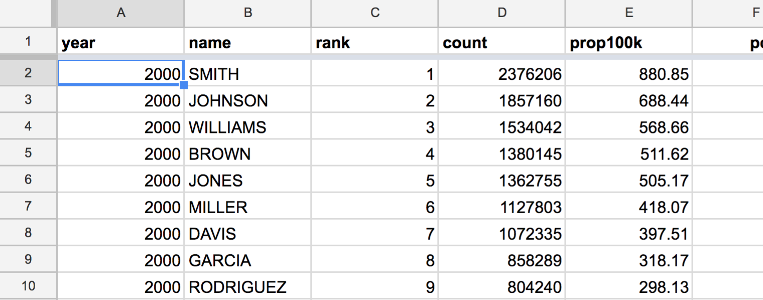
This should insert a blank column to the left of the name column. Label the column year:

Filling a column with a static value

Because we know that this entire sheet consists of Census 2000 data, we know the year value is 2000. What’s the formula to automatically fill the year column with that plain number?

Just 2000, literally. No equals sign either:

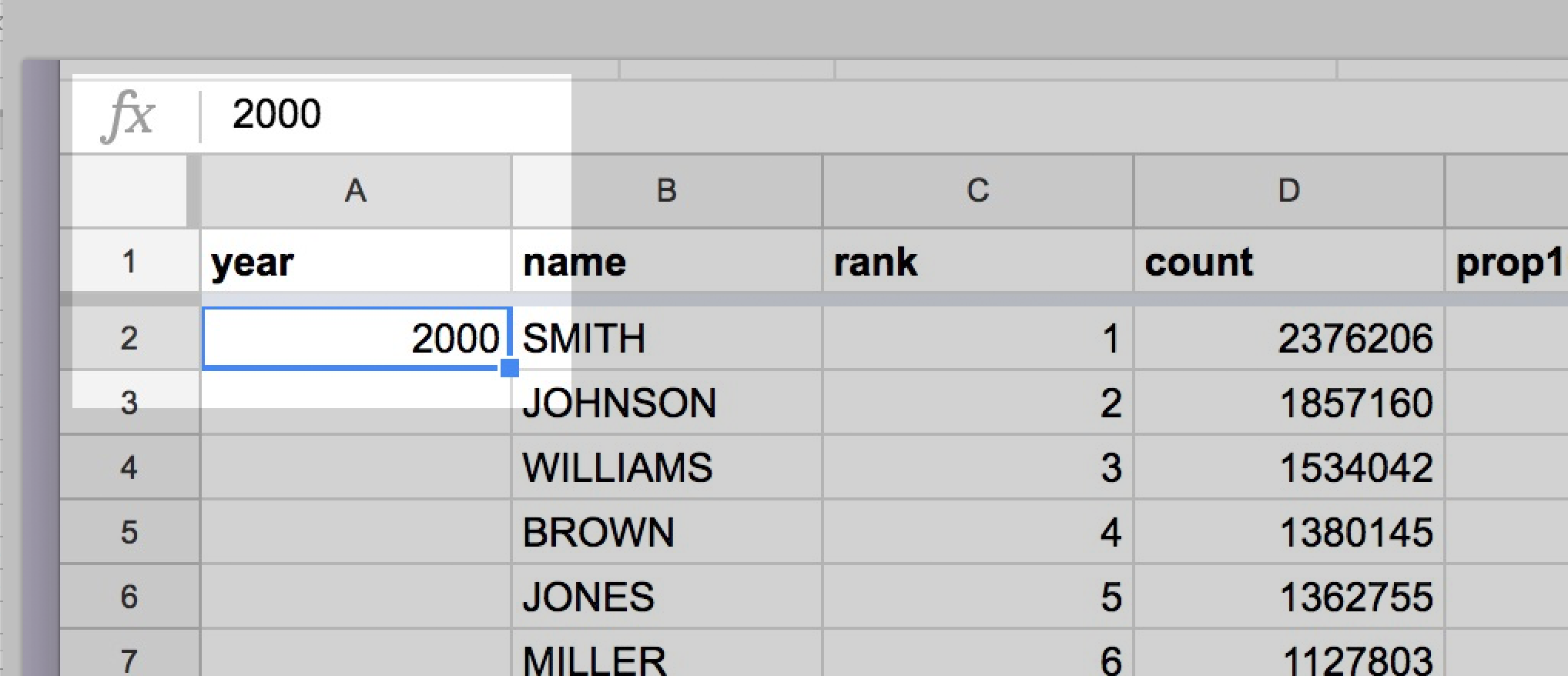
We’re obviously not interested in retyping 2000 for all the 5,000+ rows. So, if we double-click-the-blue-square in the corner of cell A2 to auto-fill the rest of the column, we get:

And that’s it for the Census 2000 data.

Combining the Census 2000 and 2010 sheets

I’ll assume that you can repeat the steps for the Census 2010 data that you used for the Census 2000 data. If you are using my Google Sheets, there should be any weirdness, such as the two different datasets having a different column schema/arrangement.

So at this point, I’m assuming you have two sheets, named “Census 2000” and “Census 2010”, respectively. And that these two sheets have a year column, filled with either 2000 or 2010, as well as about 5,000 rows each of surname data.

Let’s combine them with the fewest manual steps possible.

Create a duplicate of one of the sheets

Click either sheet’s tab to bring up a context menu, and select the Duplicate action:

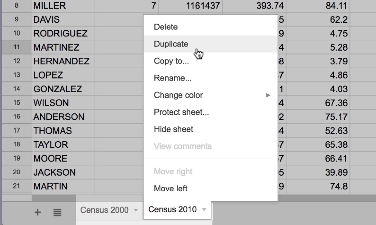
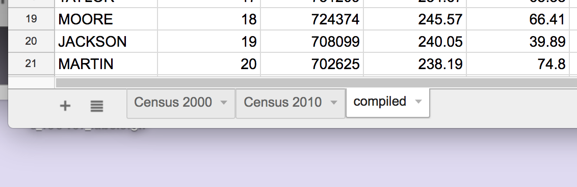
It should create a new sheet, which you should rename to something like compiled:

This will contain a sheet exactly like the one you chose to duplicate, frozen headers and all. Now select the sheet that you didn’t duplicate.

Since the compiled sheet already has headers, we want to select and copy all the rows except for the header row. The most straightforward way to do this may be to select-click row 2. Then scroll all the way to the bottom. Hold the Shift key, and select-click the row label for the final row.

Then Command/Ctrl + C to copy to clipboard. Click into the compiled. Scroll to the bottom of the compiled sheet and paste the data.

The compiled sheet may appear to have no empty rows at the bottom. Use the Add button to add a few more rows to the bottom, and then paste the Census data into the new empty rows.

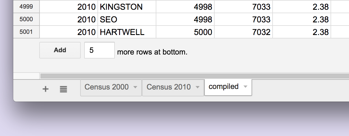
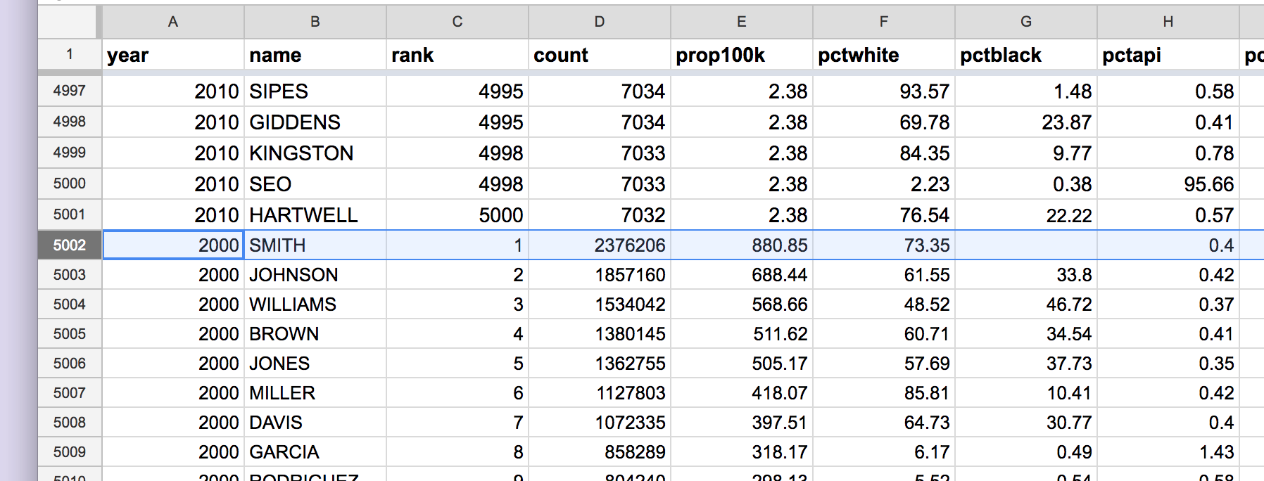
Where the two data sets were “stacked” should be pretty obvious:

Conclusion

We’ve compiled the two excerpts of the 2000 and 2010 Census datasets into one sheet, which will allow us to compare how surnames have changed between the two periods. The top 5,000 surnames per Census was a necessary step because browser-based spreadsheet can’t efficiently process the entirety of the Census data.

You can see my work on this Google Sheet:

Compiling top 5000 surnames for Census 2000 and 2010

The next lesson will be an introduction to Pivot Tables, specifically, using aggregation to quickly double-check that our compiled dataset contains the amount and scope of records we expected.