Palo Alto Pay Aggregated, 2014 vs 2016 [2017-10-16]
Attention
- Description
- Another aggregation exercise. More of a exercise in learning how to acquire data as well as analyzing it.
- Due
- 2017-10-16 23:59PM
- Slugline
padjo-2017 homework palo-alto-agg-pay your_sunet_id
Send an email with Google Sheet(s) attached. It might be easier to make a separate folder for this assignment and put all your sheets/info in there. Then give me read-permissions at dun@stanford.edu.
- Background
- Directions
- Other notes
- Answers with pivot tables
- Q4 with Pivot Tables (Palo Alto job titles with biggest pay increase)
- Step 1: Make a pivot table
- Step 2: Filter for FT-status jobs only
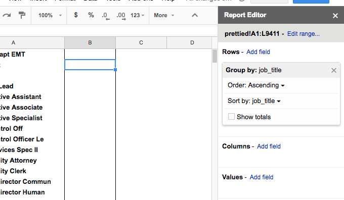
- Step 3: Add job_title as a row-pivot
- Step 4. Add year as a column-pivot
- Step 5. Add AVG of total-pay-and-benefits as a value pivot
- Step 6. Copy pivot table data, create empty sheet
- Step 7. Paste pivot table data as values only
- Step 8. Add a column calculating the difference in year salaries
- Step 9. Sort by the difference in descending order
- Q4 with Pivot Tables (Palo Alto job titles with biggest pay increase)
- Answers in SQL
Background
Public employee salary and benefits is public record, in California and in many other states. Salaries without oversight have been the stuff of several big California news investigations:
- http://www.latimes.com/about/la-times-pulitzer-prizes-htmlstory.html
- http://www.dailybreeze.com/2015/04/20/daily-breeze-wins-pulitzer-prize-for-centinela-valley-school-investigation/
The LAT’s Bell investigation spurred the state government to launch a salaries database at http://publicpay.ca.gov/.
But the state controller isn’t the only source of public salary data:
- Transparent California: http://transparentcalifornia.com/
- San Francisco Employee Compensation on Socrata: https://data.sfgov.org/City-Management-and-Ethics/Employee-Compensation/88g8-5mnd
- Reveal’s PayDay California: http://payday.revealnews.org/
Each database has a different level of detail and focus, even if they ostensibly come from the same source. Even with something as straightforward as money, there’s always different angles.
Directions
This assignment isn’t based on any particular suspicion or event. Salary data is interesting and reveals a lot about an organization. The only way to understand its nuances is to practice looking at it.
For this assignment, we’ll be using the data provided by Transparent California, for the city of Palo Alto, for the years 2014 and 2016:
- 2014 salaries for Palo Alto search page
- 2014 salaries for Palo Alto direct download
- 2016 salaries for Palo Alto search page
- 2016 salaries for Palo Alto direct download
Download the CSVs. Import it into Google Spreadsheets or Excel. Answer these questions:
- How much Palo Alto, as a whole, pays for employee salaries (total pay and benefits) in 2016 versus 2014.
- For full-time employees, the percentage of pay that went to overtime in 2016 versus 2014
- Based on employee name, how many FT employees appear to have worked for Palo Alto in 2014 and 2016 (job titles may have changed)
- Based on job title, list the 10 FT jobs that have had the highest increase in pay from 2014 to 2016.
Each of these questions should be answered with some kind of spreadsheet or pivot table. You don’t have to write a narrative for me, just send me the link to your spreadsheet that shows the calculations.
Unlike previous assignments, I’m just pointing you to the data in the wild, not making a Google spreadsheet version. If you have any trouble importing data, or figuring out spreadsheets/pivot tables, just send me an email!
Other notes
It would have been interesting to do these calculations by department. Unfortunately, if you look at the data as Transparent California provides it, it doesn’t lend itself to easy aggregation. PublicPay might have something more useful.
This assignment was originally going to use the San Francisco compensation database. Unfortunately it was too big for a spreadsheet.
Answers with pivot tables
The questions were vaguely worded such that most people came up with different answers depending on how you interpreted “total pay” (and if you caught my correction).
You can follow along with my spreadsheet here, which unlike your version, contains data for years 2011 through 2016. Just means I have an extra step of filtering for just 2014 and 2016:
Pivot table that answers Q2 - I have a feeling adding a new column to a pivot table (which I use to calculate pct overtime) is not a kosher thing to do in a real-life spreadsheet. But I do it anyway to just show the answer.
Pivot table that answers Q3 - there’s a manual step that’s not easily shown here. After doing a COUNTA calculation on ‘employee_name’ (it could be any field), and sorting that calculation in descending order so that all the names that have a COUNTA of 2 are on top, I just scroll down until I find the first name with a 1 to see that there are 717 employees who, by name, showed up in both years.
Q4 with Pivot Tables (Palo Alto job titles with biggest pay increase)
The prompt:
Based on job title, list the 10 FT jobs that have had the highest increase in pay from 2014 to 2016.
This last problem was probably the hardest for most people, so I’ll walk through every step using spreadsheets. Someday you’ll be able to do it in SQL, as I demonstrate later on in this page.
The final answer – as I’ve recreated it in my spreadsheet, can be found here.
This is similar to Q3, in which we need to find all values – this time, of ‘job_title’, not ‘employee_name’ – that exist in both years.
Step 1: Make a pivot table
This you should know how to do already.
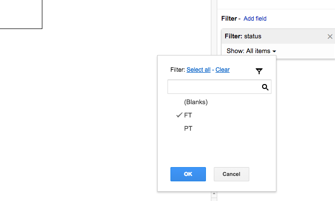
Step 2: Filter for FT-status jobs only
The question asks for jobs in which the “status” is ‘FT’. In the pivot table Report Editor, add “status” as a field and configure it so that only the ‘FT’ checkbox is checked:
Note: because my example dataset includes years other than 2014 and 2016, my pivot table also filters on the “year” field.
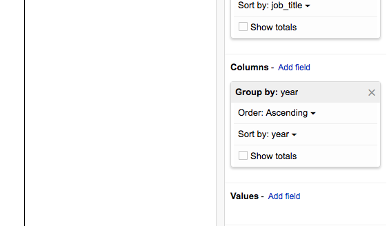
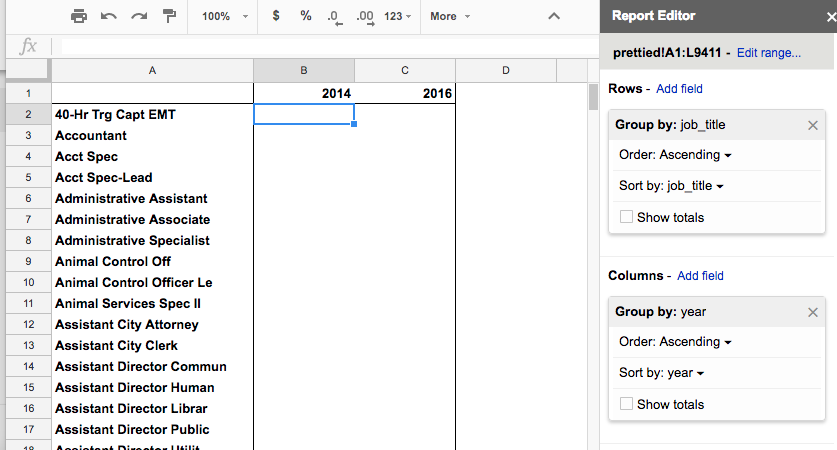
Step 4. Add year as a column-pivot
This is where the magic starts to happen:
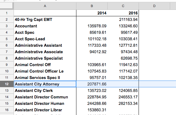
If our dataset only contains job listings in either 2014 or 2016, this column pivot will result in 2 additional columns with the header of 2014 and 2016:
Step 5. Add AVG of total-pay-and-benefits as a value pivot
We have to summarize the “total-pay-benfits” field because it is likely that some job titles have more than one person in a given year. I say to just use the AVERAGE summarization function to keep things simple:
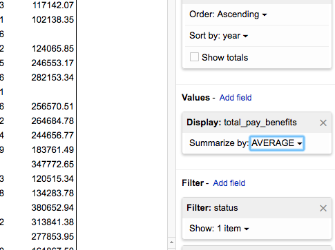
The result of choosing a value field is that the cells of our pivot table are filled with the summarization. Job titles that existed in both 2014 and 2016 have, naturally, values in both columns:
To see my spreadsheet/pivot table at this point (I’ve named it Q4-Part A), you can visit it here.
At this point, you might try to add a column after the “2016” column, in which you derive the difference between the salaries in 2016 and 2014. However, manually adding a column to a pivot table – i.e. not going through the Report Editor – is not recommended practice.
(I don’t know why, I just know through trial-and-error and gut feeling to how spreadsheets work)
More importantly for our purposes, it is impossible to sort by that ad-hoc column, which is what we need to do if we want to find the 10 jobs with the biggest increase.
Step 6. Copy pivot table data, create empty sheet
What we need to do is create a new sheet in which we can paste the pivot table values as if they were just regular old data, and add columns and sort as we like.
Select the entire pivot table with Command+A (select all) and Command+C (copy), then add a new sheet.
Step 7. Paste pivot table data as values only
You probably know Command+V as the shortcut for paste. However, we do not want to just paste what we copied from our previous pivot table, because it effectively pastes the pivot table – the values and the metadata that makes them part of a pivot table.
Instead, we just want to paste the values only of what we copied. This can be done through the menu via Edit > Paste special > Paste values only:
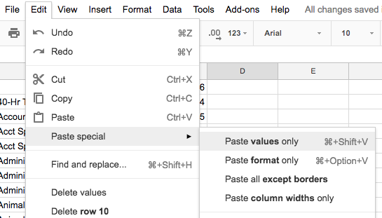
But it’s best to memorize the keyboard shortcut: Command+Shift+V
The result of Paste values only? Just good old plain text:
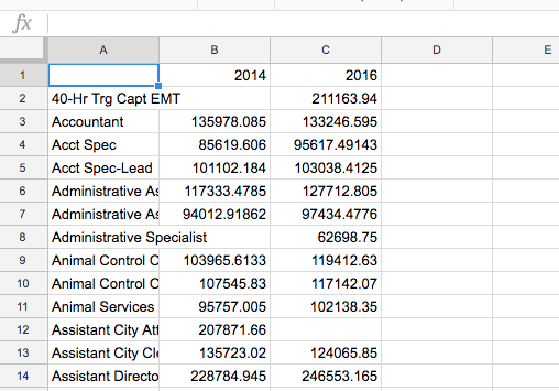
Add/freeze headers, etc, make it look like a presentable sheet if you wish.
Step 8. Add a column calculating the difference in year salaries
You know the drill. Create a new column that is derived from the other columns using a formula, e.g. =C2 - B2, and fill the column down.
However, there is a problem. For jobs that didn’t exist in 2014, the new “diff” column is calculated to be the same value as the 2016 salary, which is not what we want:
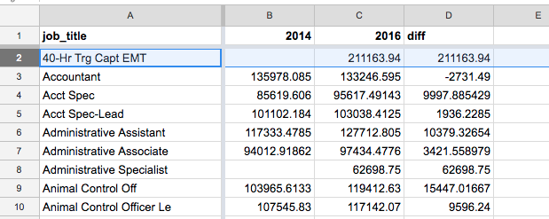
But we don’t want to consider jobs that are new in 2016. We want to find the 2014 jobs that changed the most.
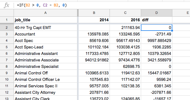
One way to do that is to use a conditional formula, i.e. if column B is blank, set column D to 0. Else, set column D to the difference of C and B.
The IF function is our friend:
=IF(B2 > 0, C2 - B2, 0)
See the difference:
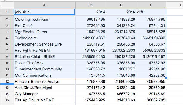
Step 9. Sort by the difference in descending order
Since the question asks for just the top 10 positions, technically we should delete the other rows. But deleting data is bad, and what’s the point of more click-work anyway? If you know a bit of SQL, you should be appreciating the LIMIT clause a bit more, as it allows us to ask for “Top X” results explicitly.
You can see my final spreadsheet here.
Answers in SQL
This assignment was assigned before we did SQL. If you want to try it in SQL, here are some answers.
Download PA salaries as a SQLite DB
You can follow along by downloading this SQLite database of Palo Alto salaries:
stash.padjo.org/data/palo-alto-salaries.sqlite
Note: It contains data for all years from 2011 to 2016, not just 2014 and 2016.
Q1 in SQL
How much Palo Alto, as a whole, pays for employee salaries (total pay and benefits) in 2016 versus 2014.
SELECT
    (SELECT
        SUM(total_pay_benefits)
    FROM salaries
    WHERE year = '2016') AS pay2016,

    (SELECT
        SUM(total_pay_benefits)
    FROM salaries
    WHERE year = '2014') AS pay2014;
| pay2016      | pay2014      |
| ------------ | ------------ |
| 163869140.16 | 147419764.12 |
Q2 in SQL
For full-time employees, the percentage of pay that went to overtime in 2016 versus 2014
The following query returns a list of years and corresponding overtime pay vs. total pay. But only for years of 2014, 2015, 2016, since the ‘FT’ designation didn’t exist in previous years:
SELECT
    year,
    ROUND(100 * SUM(overtime_pay) / SUM(total_pay), 1)
        AS pct_overtime
FROM salaries
WHERE status = 'FT'
    AND year IN ('2014', '2016')
GROUP BY year;
| year | pct_overtime |
| ---- | ------------ |
| 2014 | 7.1          |
| 2016 | 7.4          |
Q3 in SQL
Based on employee name, how many FT employees appear to have worked for Palo Alto in 2014 and 2016 (job titles may have changed)
To get something like a pivot table in which employee names with a COUNTA of 2 are listed, here’s the query:
SELECT
    employee_name,
    COUNT(*) AS ecount
FROM
    salaries
WHERE
    year IN ('2014', '2016')
         AND status = 'FT'
GROUP BY employee_name
HAVING ecount = 2
At this point, you can just count the rows to get the answer.
But if you wanted to be fancy and demonstrate your understanding of sub-queries and leave the manual counting to the computer:
SELECT
    COUNT(*)
FROM
    (SELECT
        employee_name,
        COUNT(*) AS ecount
    FROM
        salaries
    WHERE
        year IN ('2014', '2016')
             AND status = 'FT'
    GROUP BY
        employee_name
    HAVING
        ecount = 2);
Q4 in SQL (Palo Alto job titles with biggest pay increase)
Based on job title, list the 10 FT jobs that have had the highest increase in pay from 2014 to 2016.
Things are a little trickier here because, if you recall, we need to create a summation (average of total-pay-benefits) for every job title and every year. That is the kind of thing pivot tables was built for, but is intrinsically awkward (to say the least) with SQL tabular data.
At least until you understand JOINs, subqueries, self-JOINs – admittedly a cognitive load.
Here are the steps in brief: basically, we want to create 2 tables of the salary data, for 2014 and 2016 FT salaries. The queries to create those tables look like this:
SELECT
   job_title,
   AVG(total_pay_benefits) as avgtotalpay
FROM salaries
WHERE year = '2014'
    AND status = 'FT'
GROUP BY job_title;

SELECT
   job_title,
   AVG(total_pay_benefits) as avgtotalpay
FROM salaries
WHERE year = '2016'
    AND status = 'FT'
GROUP BY job_title;
But those are 2 different queries, creating 2 different result sets. How do we get those result sets to “talk” to each other?
When you are new to SQL, the easiest way to think of this kind of problem is to think of creating new tables from each of those queries. From the table salaries, we derive two sub-tables, tx and ty, for 2014 and 2016 data, respectively. They have the same schema, just different subsets of the data. If creating such sub-tables sounds wasteful and awkward, similiar to creating new sheets just to paste data from pivot table aggregations, it’s because it is. But it’s just a conceptual way to think of things.
Pretending we have these tables tx and ty, the query to JOIN the two tables, subtract their salary amounts and sort, etc, is this:
SELECT
    ty.job_title,
    ty.avgtotalpay AS pay2016,
    tx.avgtotalpay AS pay2014,
    ty.avgtotalpay - tx.avgtotalpay
        AS diff
FROM ty
INNER JOIN
    tx ON
        tx.job_title = ty.job_title
GROUP BY
    ty.job_title
ORDER BY
    diff DESC

LIMIT 10
When you get better at SQL – and thus become a lazier person overall – you hate the idea of creating these tables tx and ty manually, because you’ll see it (correctly) as annoying grunt work, and more importantly, as wasteful work for a one-time specific calculation. For example, what if the question asks for the difference between 2015 and 2017? These two throwaway tables would have to be recreated.
Once you understand subqueries, and just become less intimidated by them, you’ll be able to answer this question in a single – if very messy-looking query.
I’ll show two variations:
Subquerying and aliasing the salaries table
There is only one actual table, salaries. But by subquerying it, we effectively create new tables, which we give the aliases tx and ty:
SELECT
    ty.job_title,
    ty.avgtotalpay AS pay2016,
    tx.avgtotalpay AS pay2014,
    ty.avgtotalpay - tx.avgtotalpay
        AS diff

FROM (
        SELECT
           job_title,
           AVG(total_pay_benefits) as avgtotalpay
        FROM salaries
        WHERE year = '2014'
            AND status = 'FT'
        GROUP BY job_title)

    AS tx

INNER JOIN (
        SELECT
           job_title,
           AVG(total_pay_benefits) as avgtotalpay
        FROM salaries
        WHERE year = '2016'
            AND status = 'FT'
        GROUP BY job_title)
    AS ty
    ON ty.job_title = tx.job_title
ORDER BY
    diff DESC
LIMIT 10;
Common-table expressions
I’ll talk about “CTEs” as being the best way to do SQL even though I was completely ignorant of their existence until a chance reading of a tech blog post with the most Buzzfeedy-type headline, 10 SQL Tricks That You Didn’t Think Were Possible (under the subhed “2. Data Generation with Recursive SQL”)
(Also, CTE is a relatively new feature in SQLite and might not have been there when I first learned it)
For all intents and purposes, learning the CTE-syntax lets you organize your temp-tables-from-subqueries such that all that messy subquerying is at the top of the SQL statement. It might be almost as much code, but if you’ve done programming in other languages, you probably appreciate the ability to structure your code in this cleaner way:
WITH
    ftjobs AS (
        SELECT
            job_title,
            year,
            AVG(total_pay_benefits) AS avgtotalpay
        FROM salaries
        WHERE status = 'FT'
        GROUP BY job_title, year),

    tx AS (
        SELECT *
        FROM ftjobs
        WHERE year = '2014'),

    ty AS (
        SELECT *
        FROM ftjobs
        WHERE year = '2016')

SELECT
    ty.job_title,
    ty.avgtotalpay AS pay2016,
    tx.avgtotalpay AS pay2014,
    ty.avgtotalpay - tx.avgtotalpay
        AS diff

FROM tx

INNER JOIN ty
    ON ty.job_title = tx.job_title
ORDER BY
    diff DESC
LIMIT 10;
The results:
| job_title | pay2016 | pay2014 | diff |
|---|---|---|---|
| Metering Technician | 171888.29 | 96013.495 | 75874.795 |
| Fire Chief | 341239.24 | 273494.93 | 67744.31 |
| Mgr Electric Oprns | 231214.875 | 164298.25 | 66916.625 |
| Technologist | 207840.43 | 141188.486666667 | 66651.9433333333 |
| Development Services Dire | 290485.28 | 226119.61 | 64365.67 |
| Fire Fghtr Hz Mt EMT | 237052.283333333 | 181987.015 | 55065.2683333333 |
| Battalion Chief - Shift/E | 290127.225 | 238859.613333333 | 51267.6116666667 |
| Police Chief-Adv | 376358.98 | 328776.05 | 47582.93 |
| Superintendent Community | 188705.7 | 146360.72 | 42344.98 |
| Mgr Communications | 179848.88 | 137641.5 | 42207.38 |